Learn how to calculate a Percentage of Total in Excel. It’s widely used to normalize data and give viewers a sense of relative scale. We’ll explain when to use it, the math behind it and multiple methods for setting it up in Excel. While we’ll use the most recent version of Excel as of writing, these techniques will apply to all versions of Excel, including Excel Online,
Table of Contents
The Math to Calculate Percentage of Total
To calculate a percentage of total, divide the part by the whole. Or in Excel, divide each row by the sum of all the rows in your dataset. As a quick reminder, we’ll walk through the steps for calculating a percentage of total using an example of 10 bad apples out of 100 total apples.
1.) Identify the Part and the Whole: For Example, 10 bad apples out of 100 total apples.
2.) Divide the part by the whole: 10 bad apples / 100 total apples = 0.10
3.) Multiply the Resulting Number by 100: 0.10 * 100 = 10
4.) Apply Formatting: 10 = 10%
Now that we’ve reviewed the math involved in calculating percentage totals, let’s look at how to perform the operation in Excel.
How to Calculate Percentage of Total in Excel
To calculate a percentage total in Excel there are 4 key concepts to be aware of.
- Creating Excel Formulas to Sum and Divide
- Using Relative vs. Absolute Formulas
- Duplicating Formulas Across Multiple Rows or Columns
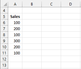
Our example uses a column of sales values. Each row is a day of sales, and we want to calculate the percentage of total for each number in our data set.
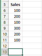
Step 1.) Calculate the Total of All Numbers
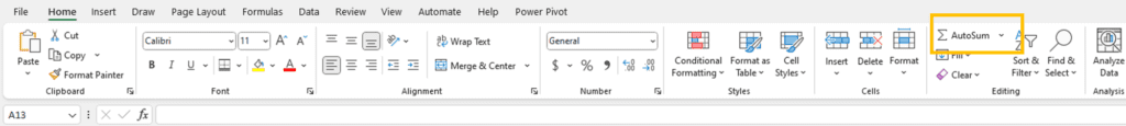
To calculate the total of all numbers in a column, we will use a sum formula. To calculate a sum, select the call that’s below the column of numbers that you wish to add. The navigate to the Home section of the Excel Ribbon, and select AutoSum. This step generates the formula to add all of the numbers above it.
Click AutoSum to automatically generate the formula to sum the numbers above the selected column.
Excel will highlight all of the cells that are about to be added together
Press enter to accept the SUM formula.

Keyboard Shortcut Tip: You can press ALT and + at the same time to automatically generate a SUM formula.
Step 2.) Calculate the percentage of total for the first row of data
To calculate the first percentage of total, create a formula using the = sign and select the first cell in the column of numbers and divide it by the total that was just calculated using the SUM formula.
To create a formula to calculate % of total follow these steps.
1.) Enter an = sign into the formula bar at the top of Excel. An = sign designates that you are entering an Excel formula and prepares it for calculation.
2.) Click on the first cell or row in the column that’s being added.
3.) Use the / symbol in Excel for division
4.) Select the Total cell that’s been calculated using your mouse.
5.) Press Enter to accept the formula

The end result will be a calculation of the percentage of total for the first row in the column of values. When complete it will look like the following:

Step 3.) Apply the Formula to all Rows in a Column
The final step in calculating a % total for all of the rows in a column is to copy the formula down so that it calculates for each cell. Before dragging the cell down to copy it to lower cells, we first have to define an absolute cell reference to the total.
Excel has two ways to define a cell reference, relative and absolute. If it’s relative, then Excel will automatically adjust the cell reference in a formula based on where a formula is moved to.
If it’s an absolute reference, the formula will point at a specific cell no matter where the formula is moved or copied to.
You can select the lower right corner of a cell and drag down. Hold the left mouse button down on the lower right triangle in the green box and drag down. The green box will get bigger and the formula will be copied into the cells below it.

However, a problem occurs because Excel will use the cell reference for the row below the starting cell for both the next row in our column, and it will also move the cell reference for the total.

This results in a #DIV/0 error because Excel can’t divide the second row in our column by a blank cell. It treats blanks like zero, and you cannot divide a number by zero.
The solution is to first define an absolute cell reference prior to copying our formula down.
To define an absolute cell reference in Excel, select a cell reference in the formula bar and Press F4 on the keyboard. The cell will be surrounded by $ signs to notate that the cell reference won’t change.

Once a value is surrounded by $ signs it won’t move as you copy the formula down to different rows.

In our example above, you can see that regardless of which row we look at, the total is still pointing to cell A13 and provides us with a % of Total for each row.
Quick Tip: You can autofill a formula down by double clicking on the small green square in the corner of a cell.
Formatting Percentage of Total Calculations
To apply percentage formatting to a number or decimal in Excel, select the cells you wish to apply the formatting to then navigate to the Number section on the Home Tab of the Excel Ribbon. Select the Percent Style button and Excel will change the formatting of each cell to a percentage. Alternatively, you can use the keyboard shortcut CTRL + SHIFT + % to automatically apply it to a selected cell.
The following screenshot highlights the percent style button in Excel.

This is what our new percentage of total column will look like after applying a percentage format to each cell.

You can select multiple cells at one time by holding down the left mouse button and drag over the cells to select them.
By using this method, you are not required to multiple a percentage by 100 to convert it from a decimal to a whole number. Excel does the hard work for you and even adds the percentage sign!
How to Make Sure a Percentage of Total Calculation is Correct in Excel
To ensure that percentage of totals are calculating correctly across all rows or columns of an Excel table, SUM the percentages column. If the SUM of all of the parts totals to 100% then the calculation is occurring correctly. You can either add the total and delete it so it isn’t presented for users or you can use the summary information at the bottom of Excel.

At the bottom of Excel, it will subtotal and show other statistics about cells that are selected. If you select all of the percentage rows, you will see that the Sum at the bottom of the page is 100%.

This method is quicker than adding an individual total cell and doesn’t require you to delete it prior to sending or printing the Excel sheet.
Conclusion
Calculating a percentage of total in Excel is a common task in Excel. You can create an excel formula to divide a row or column by a total to calculate the amount as a decima then apply percentage formatting to convert it to a percent.
Totals can quickly be calculated using the SUM formula or by clicking AutoSum in the Excel ribbon.
Once a total is calculated us an Absolute Reference to lock the reference to the total cell. Then you can either drag the formula down or double click the small green square at the bottom of a cell to automatically fill down.
Apply a percentage formula to add the % sign to numbers, and highlight the group of newly calculated cells to double check that it totals to 100% using the summary calculations at the bottom part of the Excel window.
DIV/0! errors can occur when dividing by zero, but can easily be avoided by using an IFERROR formula to tell Excel what to do when an exception occurs.